Location Test
Location testing is useful for comparing groups (also known as categories or treatments) of similar values to see if their locations are matched. In this case, location refers to a central value where all the values in a group have tendency to collect around. This is usually a mean or median of the group.
The Location Test analysis actually performs two tests, one for comparing variances between groups, and the second for comparing the location between groups. Both are useful for determining how similar or dissimilar the distribution of the groups are compared to one another.
Interpreting the Graphs
The graph produced by the Location Test produces three charts by default: Boxplots, Tukey-Kramer circles, and a Normal Quantile plot. Let’s examine these individually.
import numpy as np
import scipy.stats as st
from sci_analysis import analyze

%matplotlib inline
The Boxplots
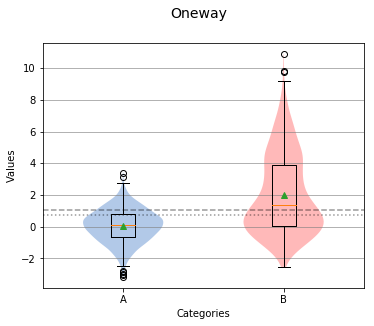
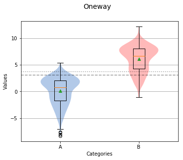
Boxplots in sci-analysis are actually a hybrid of two distribution visualization techniques, the boxplot and the violin plot. Boxplots are a good way to quickly understand a distribution, but can be misleading when the distribution is multimodal. A violin plot does a much better job at showing the local maxima and minima of a distribution.
np.random.seed(987654321)
a = st.norm.rvs(0, 1, 1000)
b = np.append(st.norm.rvs(4, 2, 500), st.norm.rvs(0, 1, 500))
analyze(
    {'A': a, 'B': b},
    circles=False,
    nqp=False,
)
Overall Statistics
------------------

Number of Groups =  2
Total            =  2000
Grand Mean       =  1.0413
Pooled Std Dev   =  1.9068
Grand Median     =  0.7279


Group Statistics
----------------

n             Mean          Std Dev       Min           Median        Max           Group
--------------------------------------------------------------------------------------------------
1000           0.0551        1.0287       -3.1586        0.0897        3.4087       A
1000           2.0275        2.4926       -2.5414        1.3661        10.8915      B


Levene Test
-----------

alpha   =  0.0500
W value =  513.4363
p value =  0.0000

HA: Variances are not equal


Mann Whitney U Test
-------------------

alpha   =  0.0500
u value =  263634.0000
p value =  0.0000

HA: Locations are not matched
In the center of each box is a red line and green triangle. The green triangle represents the mean of the group while the red line represents the median, sometimes referred to as the second quartile (Q2) or 50% line.
The boxplot graph also shows a short dotted line and long dotted line that represent the grand median and grand mean respectively.
np.random.seed(987654321)
a = np.append(st.norm.rvs(2, 1, 500), st.norm.rvs(-2, 2, 500))
b = np.append(st.norm.rvs(8, 1, 500), st.norm.rvs(4, 2, 500))
analyze(
    {'A': a, 'B': b},
    circles=False,
    nqp=False,
)
Overall Statistics
------------------

Number of Groups =  2
Total            =  2000
Grand Mean       =  3.0982
Pooled Std Dev   =  2.4841
Grand Median     =  3.7150


Group Statistics
----------------

n             Mean          Std Dev       Min           Median        Max           Group
--------------------------------------------------------------------------------------------------
1000           0.0957        2.5307       -8.3172        0.7375        5.4087       A
1000           6.1006        2.4365       -1.0829        6.6925        12.1766      B


Levene Test
-----------

alpha   =  0.0500
W value =  0.6238
p value =  0.4297

H0: Variances are equal


Mann Whitney U Test
-------------------

alpha   =  0.0500
u value =  43916.0000
p value =  0.0000

HA: Locations are not matched
Tukey-Kramer Circles
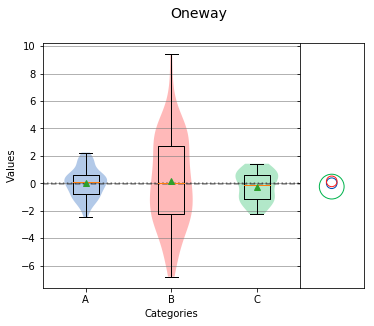
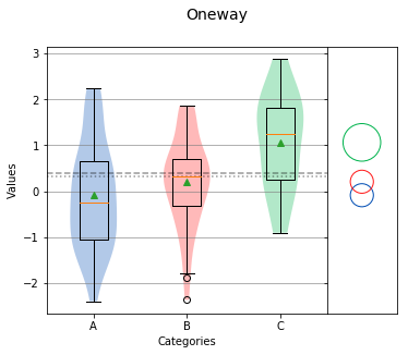
Tukey-Kramer Circles, also referred to as comparison circles are based on the Tukey HSD test. Each circle is centered on the mean of each group and the radius of the circle is calculated from the mean standard error and size of the group. In this case, the radius is proportional to the standard error and inversely proportional to the size of the group. Therefore, a higher variation or smaller group size will produce a larger circle.
np.random.seed(987654321)
a = st.norm.rvs(0, 1, 100)
b = st.norm.rvs(0, 3, 100)
c = st.norm.rvs(0, 1, 20)
analyze(
    {'A': a, 'B': b, 'C': c},
    nqp=False,
)
Overall Statistics
------------------

Number of Groups =  3
Total            =  220
Grand Mean       = -0.0286
Pooled Std Dev   =  2.3353
Grand Median     =  0.0394


Group Statistics
----------------

n             Mean          Std Dev       Min           Median        Max           Group
--------------------------------------------------------------------------------------------------
100            0.0083        1.0641       -2.4718        0.0761        2.2466       A
100            0.1431        3.2552       -6.8034        0.0394        9.4199       B
20            -0.2373        1.0830       -2.2349       -0.1229        1.4290       C


Bartlett Test
-------------

alpha   =  0.0500
T value =  117.7279
p value =  0.0000

HA: Variances are not equal


Kruskal-Wallis
--------------

alpha   =  0.0500
h value =  0.2997
p value =  0.8608

H0: Group means are matched
If circles of different groups are mostly overlapping, the means of those groups are likely matched. However, if circles are not touching each other or only partly overlap, the means of those groups are likely different.
np.random.seed(987654321)
a = st.norm.rvs(0, 1, 50)
b = st.norm.rvs(0.1, 1, 50)
c = st.norm.rvs(1, 1, 20)
analyze(
    {'A': a, 'B': b, 'C': c},
    nqp=False,
)
Overall Statistics
------------------

Number of Groups =  3
Total            =  120
Grand Mean       =  0.3935
Pooled Std Dev   =  1.0608
Grand Median     =  0.3123


Group Statistics
----------------

n             Mean          Std Dev       Min           Median        Max           Group
--------------------------------------------------------------------------------------------------
50            -0.0891        1.1473       -2.4036       -0.2490        2.2466       A
50             0.2057        0.9758       -2.3718        0.3123        1.8617       B
20             1.0637        1.0391       -0.9072        1.2480        2.8849       C


Bartlett Test
-------------

alpha   =  0.0500
T value =  1.2811
p value =  0.5270

H0: Variances are equal


Oneway ANOVA
------------

alpha   =  0.0500
f value =  8.4504
p value =  0.0004

HA: Group means are not matched
Normal Quantile Plot
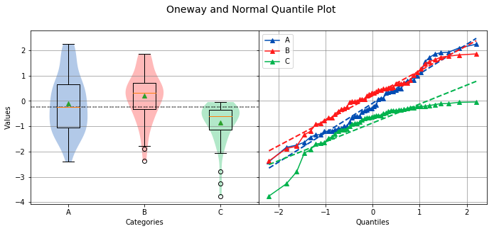
A Normal Quantile Plot is a specific type of Quantile-Quantile (Q-Q) plot where the quantiles on the x-axis correspond to the quantiles of the normal distribution. In the case of the Normal Quantile Plot, one quantile corresponds to one standard deviation.
If the plotted points for a group on the Normal Quantile Plot closely resemble a straight line (regardless of slope), then the group is normally distributed. In the example below, group C is not normally distributed, as seen by it’s downward curved shape on the Normal Quantile Plot.
np.random.seed(987654321)
a = st.norm.rvs(0, 1, size=50)
b = st.norm.rvs(0.1, 1, size=50)
c = st.weibull_max.rvs(0.95, size=50)
analyze(
    {'A': a, 'B': b, 'C': c},
    circles=False,
)
Overall Statistics
------------------

Number of Groups =  3
Total            =  150
Grand Mean       = -0.2507
Pooled Std Dev   =  0.9868
Grand Median     = -0.2490


Group Statistics
----------------

n             Mean          Std Dev       Min           Median        Max           Group
--------------------------------------------------------------------------------------------------
50            -0.0891        1.1473       -2.4036       -0.2490        2.2466       A
50             0.2057        0.9758       -2.3718        0.3123        1.8617       B
50            -0.8687        0.8078       -3.7612       -0.6117       -0.0409       C


Levene Test
-----------

alpha   =  0.0500
W value =  4.5142
p value =  0.0125

HA: Variances are not equal


Kruskal-Wallis
--------------

alpha   =  0.0500
h value =  28.3558
p value =  0.0000

HA: Group means are not matched
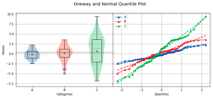
The slope of the data points on the Normal Quantile Plot indicate the relative variance of a particular group compared to the other groups.
np.random.seed(987654321)
a = st.norm.rvs(0, 1, 50)
b = st.norm.rvs(0, 2, 50)
c = st.norm.rvs(0, 3, 50)
analyze(
    {'A': a, 'B': b, 'C': c},
    circles=False,
)
Overall Statistics
------------------

Number of Groups =  3
Total            =  150
Grand Mean       =  0.3013
Pooled Std Dev   =  2.4717
Grand Median     =  0.4247


Group Statistics
----------------

n             Mean          Std Dev       Min           Median        Max           Group
--------------------------------------------------------------------------------------------------
50            -0.0891        1.1473       -2.4036       -0.2490        2.2466       A
50             0.2113        1.9515       -4.9435        0.4247        3.5233       B
50             0.7816        3.6335       -6.8034        1.3194        9.4199       C


Bartlett Test
-------------

alpha   =  0.0500
T value =  60.0600
p value =  0.0000

HA: Variances are not equal


Kruskal-Wallis
--------------

alpha   =  0.0500
h value =  3.4335
p value =  0.1796

H0: Group means are matched
Interpreting the Statistics
When performing a Location Test analysis, two statistics tables are given, the Overall Statistics and the Group Statistics.
The Overall Statistics shows the number of groups in the dataset, total number of data points in the dataset, Grand Mean, Grand Median, and Pooled Standard Deviation.
The Group Statistics list summary statistics for each group in a table. The summary statistics shown are the number of data points in the group (n), the Mean, Standard Deviation, Minimum, Median, Maximum, and group name.
The remaining two statistics are both Hypothesis Tests. The first test attempts to determine if the variances of each group are matched or not. The second test attempts to determine if the locations of each group are matched or not. Each hypothesis test shows the significance level (alpha), test statistic, and p-value. The hypothesis test used depends on a few different factors. The test for equal variance is fairly simple and depends on whether the all the data points in the dataset are normally distributed or not. If normally distributed, the Bartlett Test is used, otherwise the Levene Test is used.
The logic for determining which hypothesis test to use for checking location is more complex and depends on the number of groups, whether the data points in the dataset are normally distributed, and the size of the smallest group.
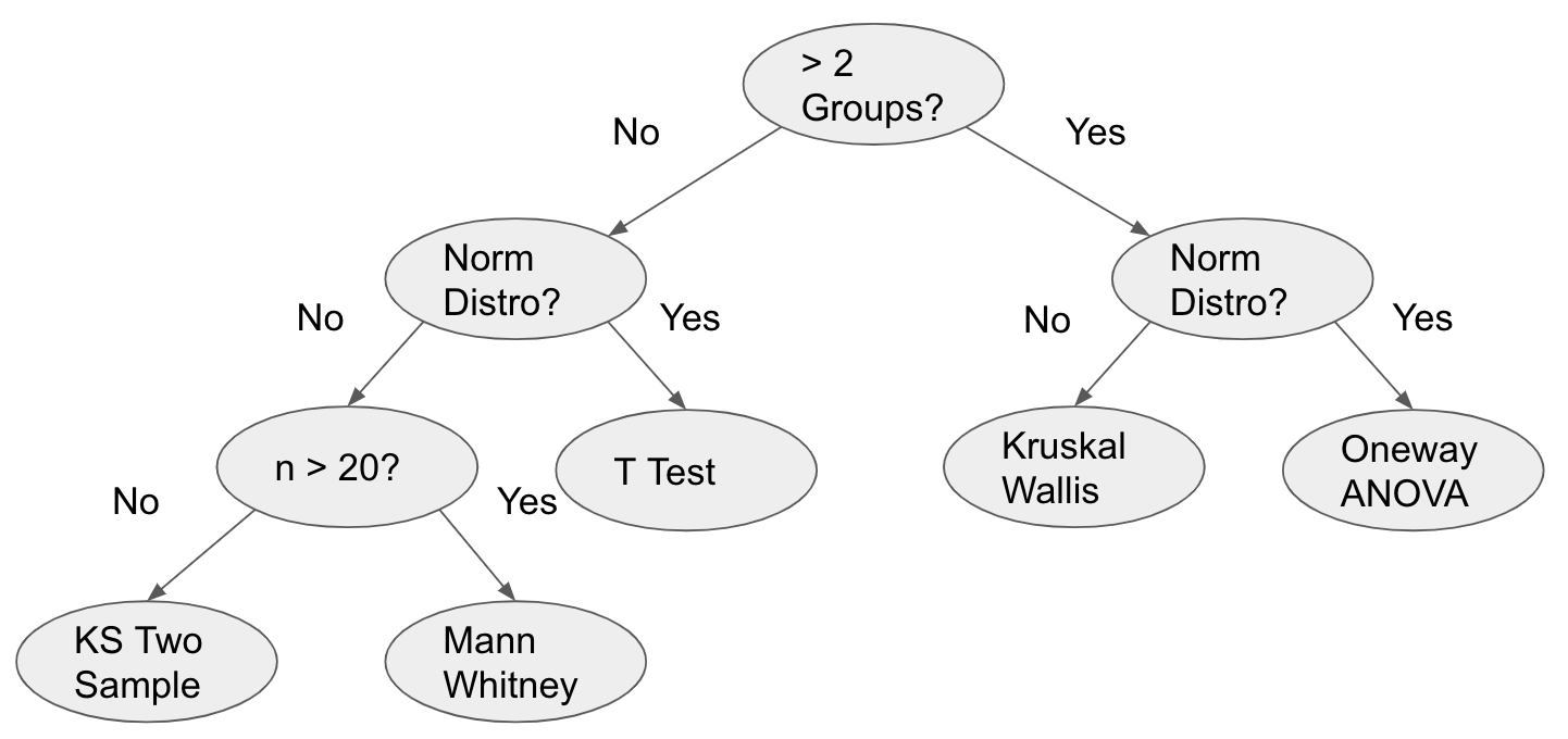
The five possible hypothesis tests from most sensitive to least sensitive are:
The last thing shown for each hypothesis test is the statement of the null hypothesis or alternative hypothesis. Each hypothesis has a null hypothesis that is assumed to be true. If the p-value of the test is lower than the significance level (alpha) of the test, the null hypothesis is rejected and the alternative hypothesis is stated. When the null hypothesis is rejected, it means that the likelihood of the outcome occurring by chance is significantly low enough that it is likely true.
Because the conclusion of hypothesis testing depends on an arbitrarily chosen significance level of 0.05, they should be taken with a bit of caution. This is why sci-analysis goes to lengths to try to use the most appropriate test given the supplied data and also pairs the test with graphs for a second source of truth.
Usage
Stacked Data
-
analyze(sequence, groups[, nqp=True, circles=True, alpha=0.05, title=’Oneway’, categories=’Categories’, xname=’Categories’, name=’Values’, yname=’Values’, save_to=None])¶ Performs a location test of numeric, stacked data.
Parameters: - sequence (array-like) – The array-like object to analyze. It can be a list, tuple, numpy array or pandas Series of numeric values.
- groups (array-like) – An array-like of categorical values to group numeric values in sequence by. The values in groups correspond to the value at the same index in sequence. For this reason, the length of sequence and groups should be equal.
- nqp (bool) – Display the accompanying Normal Quantile Plot if True. The default value is True.
- circles (bool) – Display the Tukey-Kramer circles if True. The default value is True.
- alpha (float) – The significance level to use for hypothesis tests. The default value is 0.05.
- title (str) – The title of the graph.
- categories (str) – The label of the categories (groups) to be displayed along the x-axis of the graph.
- xname (str) – Alias for categories.
- name (str) – The label of the values in sequence to be displayed on the y-axis of the graph.
- yname (str) – Alias for name.
- or None save_to (str) – The path to the file where the graph will be saved.
Unstacked Data
-
analyze(sequences[, groups=None, nqp=True, circles=True, alpha=0.05, title=’Oneway’, categories=’Categories’, xname=’Categories’, name=’Values’, yname=’Values’, save_to=None]) Performs a location test of numeric, unstacked data.
Parameters: - or dict sequences (array-like) – The object to analyze. If sequences is a dictionary, the keys will be used as the group names and the groups argument will be ignored. If sequences is an array-like, its values should be array-likes for each group to analyze. If groups is None, numbers will automatically be assigned as category names for each array-like in sequences.
- groups (list) – A list of categories to group values in sequences by. The order of values in groups should match the array-like values in sequences.
- nqp (bool) – Display the accompanying Normal Quantile Plot if True. The default value is True.
- circles (bool) – Display the Tukey-Kramer circles if True. The default value is True.
- alpha (float) – The significance level to use for hypothesis tests. The default value is 0.05.
- title (str) – The title of the graph.
- categories (str) – The label of the categories (groups) to be displayed along the x-axis of the graph.
- xname (str) – Alias for categories.
- name (str) – The label of the values in sequence to be displayed on the y-axis of the graph.
- yname (str) – Alias for name.
- or None save_to (str) – The path to the file where the graph will be saved.
Argument Examples
Let’s first import sci-analysis and setup some variables to use in these examples.
# Create sequence and groups from random variables for stacked data examples.
stacked = st.norm.rvs(2, 0.45, size=3000)
vals = 'ABCD'
stacked_groups = []
for _ in range(3000):
    stacked_groups.append(vals[np.random.randint(0, 4)])
sequence, groups
When analyzing stacked data, both sequence and groups are required.
analyze(
    stacked,
    groups=stacked_groups,
)

Overall Statistics
------------------

Number of Groups =  4
Total            =  3000
Grand Mean       =  2.0118
Pooled Std Dev   =  0.4558
Grand Median     =  2.0174


Group Statistics
----------------

n             Mean          Std Dev       Min           Median        Max           Group
--------------------------------------------------------------------------------------------------
720            2.0211        0.4667        0.6218        2.0240        3.5506       A
736            2.0126        0.4729        0.6281        2.0228        3.5339       B
782            1.9991        0.4403        0.5786        2.0120        3.4248       C
762            2.0143        0.4439        0.6396        2.0046        3.8397       D


Bartlett Test
-------------

alpha   =  0.0500
T value =  5.7422
p value =  0.1248

H0: Variances are equal


Oneway ANOVA
------------

alpha   =  0.0500
f value =  0.3117
p value =  0.8169

H0: Group means are matched
sequences
When analyzing unstacked data, sequences can be a dictionary or an array-like of array-likes.
# Create sequences from random variables for unstacked data examples.
np.random.seed(987654321)
a = st.norm.rvs(2, 0.45, size=750)
b = st.norm.rvs(2, 0.45, size=750)
c = st.norm.rvs(2, 0.45, size=750)
d = st.norm.rvs(2, 0.45, size=750)
If sequences is an array-like of array-likes, and groups is None, category labels will be automatically generated starting at 1.
analyze([a, b, c, d])

Overall Statistics
------------------

Number of Groups =  4
Total            =  3000
Grand Mean       =  2.0149
Pooled Std Dev   =  0.4564
Grand Median     =  2.0219


Group Statistics
----------------

n             Mean          Std Dev       Min           Median        Max           Group
--------------------------------------------------------------------------------------------------
750            2.0234        0.4679        0.5786        2.0328        3.5339       1
750            2.0006        0.4553        0.6281        2.0110        3.5506       2
750            2.0538        0.4446        0.8564        2.0512        3.8397       3
750            1.9819        0.4575        0.6218        1.9780        3.2952       4


Bartlett Test
-------------

alpha   =  0.0500
T value =  1.9719
p value =  0.5783

H0: Variances are equal


Oneway ANOVA
------------

alpha   =  0.0500
f value =  3.4508
p value =  0.0159

HA: Group means are not matched
If sequences is a dictionary, the keys will be used as category labels. .. note:: When sequences is a dictionary, the categories will not necessarily be shown in order.
analyze({'A': a, 'B': b, 'C': c, 'D': d})

Overall Statistics
------------------

Number of Groups =  4
Total            =  3000
Grand Mean       =  2.0149
Pooled Std Dev   =  0.4564
Grand Median     =  2.0219


Group Statistics
----------------

n             Mean          Std Dev       Min           Median        Max           Group
--------------------------------------------------------------------------------------------------
750            2.0234        0.4679        0.5786        2.0328        3.5339       A
750            2.0006        0.4553        0.6281        2.0110        3.5506       B
750            2.0538        0.4446        0.8564        2.0512        3.8397       C
750            1.9819        0.4575        0.6218        1.9780        3.2952       D


Bartlett Test
-------------

alpha   =  0.0500
T value =  1.9719
p value =  0.5783

H0: Variances are equal


Oneway ANOVA
------------

alpha   =  0.0500
f value =  3.4508
p value =  0.0159

HA: Group means are not matched
groups
If analyzing stacked data, groups should be an array-like with the same length as sequence. If analyzing unstacked data, groups should be the same length as sequences and all values in lgroups should be unique.
analyze(
    [a, b, c, d],
    groups=['A', 'B', 'C', 'D'],
)

Overall Statistics
------------------

Number of Groups =  4
Total            =  3000
Grand Mean       =  2.0149
Pooled Std Dev   =  0.4564
Grand Median     =  2.0219


Group Statistics
----------------

n             Mean          Std Dev       Min           Median        Max           Group
--------------------------------------------------------------------------------------------------
750            2.0234        0.4679        0.5786        2.0328        3.5339       A
750            2.0006        0.4553        0.6281        2.0110        3.5506       B
750            2.0538        0.4446        0.8564        2.0512        3.8397       C
750            1.9819        0.4575        0.6218        1.9780        3.2952       D


Bartlett Test
-------------

alpha   =  0.0500
T value =  1.9719
p value =  0.5783

H0: Variances are equal


Oneway ANOVA
------------

alpha   =  0.0500
f value =  3.4508
p value =  0.0159

HA: Group means are not matched
nqp
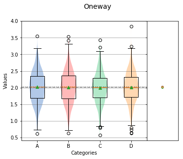
Controls whether the Normal Quantile Plot is displayed or not. The default value is True.
analyze(
    stacked,
    groups=stacked_groups,
    nqp=False,
)
Overall Statistics
------------------

Number of Groups =  4
Total            =  3000
Grand Mean       =  2.0118
Pooled Std Dev   =  0.4558
Grand Median     =  2.0174


Group Statistics
----------------

n             Mean          Std Dev       Min           Median        Max           Group
--------------------------------------------------------------------------------------------------
720            2.0211        0.4667        0.6218        2.0240        3.5506       A
736            2.0126        0.4729        0.6281        2.0228        3.5339       B
782            1.9991        0.4403        0.5786        2.0120        3.4248       C
762            2.0143        0.4439        0.6396        2.0046        3.8397       D


Bartlett Test
-------------

alpha   =  0.0500
T value =  5.7422
p value =  0.1248

H0: Variances are equal


Oneway ANOVA
------------

alpha   =  0.0500
f value =  0.3117
p value =  0.8169

H0: Group means are matched
circles
Controls whether the Tukey-Kramer circles are displayed or not. The default value is True.
analyze(
    stacked,
    groups=stacked_groups,
    circles=False,
)
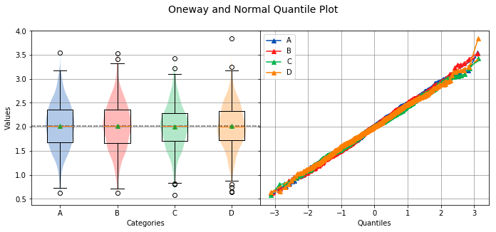
Overall Statistics
------------------

Number of Groups =  4
Total            =  3000
Grand Mean       =  2.0118
Pooled Std Dev   =  0.4558
Grand Median     =  2.0174


Group Statistics
----------------

n             Mean          Std Dev       Min           Median        Max           Group
--------------------------------------------------------------------------------------------------
720            2.0211        0.4667        0.6218        2.0240        3.5506       A
736            2.0126        0.4729        0.6281        2.0228        3.5339       B
782            1.9991        0.4403        0.5786        2.0120        3.4248       C
762            2.0143        0.4439        0.6396        2.0046        3.8397       D


Bartlett Test
-------------

alpha   =  0.0500
T value =  5.7422
p value =  0.1248

H0: Variances are equal


Oneway ANOVA
------------

alpha   =  0.0500
f value =  0.3117
p value =  0.8169

H0: Group means are matched
alpha
Sets the significance level to use for hypothesis testing.
analyze(
    stacked,
    groups=stacked_groups,
    alpha=0.01,
)

Overall Statistics
------------------

Number of Groups =  4
Total            =  3000
Grand Mean       =  2.0118
Pooled Std Dev   =  0.4558
Grand Median     =  2.0174


Group Statistics
----------------

n             Mean          Std Dev       Min           Median        Max           Group
--------------------------------------------------------------------------------------------------
720            2.0211        0.4667        0.6218        2.0240        3.5506       A
736            2.0126        0.4729        0.6281        2.0228        3.5339       B
782            1.9991        0.4403        0.5786        2.0120        3.4248       C
762            2.0143        0.4439        0.6396        2.0046        3.8397       D


Bartlett Test
-------------

alpha   =  0.0100
T value =  5.7422
p value =  0.1248

H0: Variances are equal


Oneway ANOVA
------------

alpha   =  0.0100
f value =  0.3117
p value =  0.8169

H0: Group means are matched
title
The title of the distribution to display above the graph.
analyze(
    stacked,
    groups=stacked_groups,
    title='This is a Title',
)

Overall Statistics
------------------

Number of Groups =  4
Total            =  3000
Grand Mean       =  2.0118
Pooled Std Dev   =  0.4558
Grand Median     =  2.0174


Group Statistics
----------------

n             Mean          Std Dev       Min           Median        Max           Group
--------------------------------------------------------------------------------------------------
720            2.0211        0.4667        0.6218        2.0240        3.5506       A
736            2.0126        0.4729        0.6281        2.0228        3.5339       B
782            1.9991        0.4403        0.5786        2.0120        3.4248       C
762            2.0143        0.4439        0.6396        2.0046        3.8397       D


Bartlett Test
-------------

alpha   =  0.0500
T value =  5.7422
p value =  0.1248

H0: Variances are equal


Oneway ANOVA
------------

alpha   =  0.0500
f value =  0.3117
p value =  0.8169

H0: Group means are matched
categories, xname
The name of the category labels to display on the x-axis.
analyze(
    stacked,
    groups=stacked_groups,
    categories='Generated Categories',
)

Overall Statistics
------------------

Number of Groups =  4
Total            =  3000
Grand Mean       =  2.0118
Pooled Std Dev   =  0.4558
Grand Median     =  2.0174


Group Statistics
----------------

n             Mean          Std Dev       Min           Median        Max           Group
--------------------------------------------------------------------------------------------------
720            2.0211        0.4667        0.6218        2.0240        3.5506       A
736            2.0126        0.4729        0.6281        2.0228        3.5339       B
782            1.9991        0.4403        0.5786        2.0120        3.4248       C
762            2.0143        0.4439        0.6396        2.0046        3.8397       D


Bartlett Test
-------------

alpha   =  0.0500
T value =  5.7422
p value =  0.1248

H0: Variances are equal


Oneway ANOVA
------------

alpha   =  0.0500
f value =  0.3117
p value =  0.8169

H0: Group means are matched
analyze(
    stacked,
    groups=stacked_groups,
    xname='Generated Categories',
)

Overall Statistics
------------------

Number of Groups =  4
Total            =  3000
Grand Mean       =  2.0118
Pooled Std Dev   =  0.4558
Grand Median     =  2.0174


Group Statistics
----------------

n             Mean          Std Dev       Min           Median        Max           Group
--------------------------------------------------------------------------------------------------
720            2.0211        0.4667        0.6218        2.0240        3.5506       A
736            2.0126        0.4729        0.6281        2.0228        3.5339       B
782            1.9991        0.4403        0.5786        2.0120        3.4248       C
762            2.0143        0.4439        0.6396        2.0046        3.8397       D


Bartlett Test
-------------

alpha   =  0.0500
T value =  5.7422
p value =  0.1248

H0: Variances are equal


Oneway ANOVA
------------

alpha   =  0.0500
f value =  0.3117
p value =  0.8169

H0: Group means are matched
name, yname
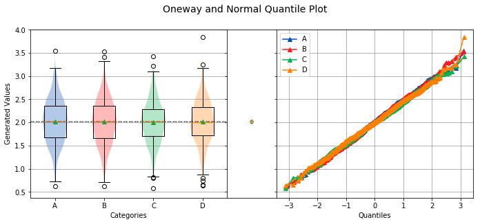
The label to display on the y-axis.
analyze(
    stacked,
    groups=stacked_groups,
    name='Generated Values',
)
Overall Statistics
------------------

Number of Groups =  4
Total            =  3000
Grand Mean       =  2.0118
Pooled Std Dev   =  0.4558
Grand Median     =  2.0174


Group Statistics
----------------

n             Mean          Std Dev       Min           Median        Max           Group
--------------------------------------------------------------------------------------------------
720            2.0211        0.4667        0.6218        2.0240        3.5506       A
736            2.0126        0.4729        0.6281        2.0228        3.5339       B
782            1.9991        0.4403        0.5786        2.0120        3.4248       C
762            2.0143        0.4439        0.6396        2.0046        3.8397       D


Bartlett Test
-------------

alpha   =  0.0500
T value =  5.7422
p value =  0.1248

H0: Variances are equal


Oneway ANOVA
------------

alpha   =  0.0500
f value =  0.3117
p value =  0.8169

H0: Group means are matched
analyze(
    stacked,
    groups=stacked_groups,
    yname='Generated Values',
)

Overall Statistics
------------------

Number of Groups =  4
Total            =  3000
Grand Mean       =  2.0118
Pooled Std Dev   =  0.4558
Grand Median     =  2.0174


Group Statistics
----------------

n             Mean          Std Dev       Min           Median        Max           Group
--------------------------------------------------------------------------------------------------
720            2.0211        0.4667        0.6218        2.0240        3.5506       A
736            2.0126        0.4729        0.6281        2.0228        3.5339       B
782            1.9991        0.4403        0.5786        2.0120        3.4248       C
762            2.0143        0.4439        0.6396        2.0046        3.8397       D


Bartlett Test
-------------

alpha   =  0.0500
T value =  5.7422
p value =  0.1248

H0: Variances are equal


Oneway ANOVA
------------

alpha   =  0.0500
f value =  0.3117
p value =  0.8169

H0: Group means are matched